1 Introduction

The multivariate normal distribution arises frequently and has a wide range of applications in fields such as multivariate regression, Bayesian statistics and the analysis of Brownian motion. One motivation to deal with moments of the truncated multivariate normal distribution comes from the analysis of special financial derivatives (“auto-callables” or “Expresszertifikate”) in Germany. These products can expire early depending on some restrictions of the underlying trajectory, if the underlying value is above or below certain call levels. In the framework of Brownian motion the finite-dimensional distributions for log returns at any $d$ points in time are multivariate normal. When some of the multinormal variates $\bfX =(x_1,\ldots ,x_d)' \sim N(\bfmu ,\mathbf {\Sigma })$ are subject to inequality constraints (e.g. $a_i \le x_i \le b_i$), this results in truncated multivariate normal distributions.

Several types of truncations and their moment calculation have been described so far, for example the one-sided rectangular truncation $\bfx \ge \bfa $ (Tallis, 1961), the rather unusual elliptical and radial truncations $\bfa \le \bfx ' \bfR \bfx \le \bfb $ (Tallis, 1963) and the plane truncation $\bfC \bfx \ge \bfp $ (Tallis, 1965). Linear constraints like $\bfa \le \bfC \bfx \le \bfb $ can often be reduced to rectangular truncation by transformation of the variables (in case of a full rank matrix $\bfC $ : $\bfa ^{*} = \bfC ^{-1} \bfa \le \bfx \le \bfC ^{-1} \bfb = \bfb ^{*}$), which makes the double rectangular truncation $\bfa \le \bfx \le \bfb $ especially important.

The existing works on moment calculations differ in the number of variables they consider (univariate, bivariate, multivariate) and the types of rectangular truncation they allow (single vs. double truncation). Single or one-sided truncation can be either from above ($\bfx \le \bfa $) or below ($\bfx \ge \bfa $), but only on one side for all variables, whereas double truncation $\bfa \le \bfx \le \bfb $ can have both lower and upper truncation points. Other distinguishing features of previous works are further limitations or restrictions they impose on the type of distribution (e.g. zero mean) and the methods they use to derive the results (e.g. direct integration or moment-generating function).

Rosenbaum (1961) gave an explicit formula for the moments of the bivariate case with single truncation from below in both variables by direct integration. His results for the bivariate normal distribution have been extended by Shah and Parikh (1964), Regier and Hamdan (1971) and Muthen (1990) to double truncation.

For the multivariate case, Tallis (1961) derived an explicit expression for the first two moments in case of a singly truncated multivariate normal density with zero mean vector and the correlation matrix $\bfR $ using the moment generating function. Amemiya (1974) and Lee (1979) extended the Tallis (1961) derivation to a general covariance matrix $\bfSi $ and also evaluated the relationship between the first two moments. Gupta and Tracy (1976) and Lee (1983) gave very simple recursive relationships between moments of any order for the doubly truncated case. However, except for the mean, there are fewer equations than parameters. Therefore, these recurrent conditions do not uniquely identify moments of order $\ge 2$ and are not sufficient for the computation of the variance and other higher order moments.

Table 1 summarizes our survey of existing publications dealing with the computation of truncated moments and their limitations.

Even though the rectangular truncation $\bfa \le \bfx \le \bfb $ can be found in many situations, no explicit moment formulas for the truncated mean and variance in the general multivariate case of double truncation from below and/or above have been presented so far in the literature and are readily apparent. The contribution of this paper is to derive these formulas for the first two truncated moments and to extend and generalize existing results on moment calculations from especially Tallis (1961), Lee (1983), Leppard and Tallis (1989), and Muthen (1990). Besides, we also refer Kan and Robotti (2017) and Arismendi (2013) for the moment computation of folded and truncated multivariate normal distribution. However, for moments computation for skewed and extended skew normal distribution, we refer Kan and Robotti (2017) and Arellano-Valle and Genton (2005). In the sequel, we also make a note on the existing R package ”MomTrunc” (see Galarza C.E. & V.H., 2021) for numerical computation of moments of folded and truncated multivariate normal and Student’s t-distribution. However, the aforementioned package also suggests the ”tmvtnorm” package (e.g., Wilhelm & Manjunath, 2012), which is solely based on the results presented in this note. Finally, we also refer Genz (1992) for the numerical computation for the multivariate normal probabilities.

The rest of this paper is organized as follows. Section 2 presents the moment generating function (m.g.f) for the doubly truncated multivariate normal case. In Section 3, we derive the first and second moments by differentiating the m.g.f. These results are completed in Section 4 by giving a formula for computing the bivariate marginal density. In Section 5, we present two numerical examples and compare our results with simulation results. Section 6 links our results to the theory of graphical models and derives some properties of the inverse covariance matrix. Finally, Section 7 summarizes our results and gives an outlook for further research.

2 Moment Generating Function

The $d$–dimensional normal density with location parameter vector $\bfmu \in \mathbb {R}^d$ and non-singular covariance matrix $\bfSi $ is given by

The pertaining distribution function is denoted by $\Phi _{\sbmu ,\sbsi } (\bfx )$. Correspondingly, the multivariate truncated normal density, truncated at $\bfa $ and $\bfb $, in $\mathbb {R}^d$, is defined as Denote $\alpha = P\left \{\bfa \leq \bfX \leq \bfb \right \}$ as the fraction after truncation.

The moment generating function of a $d$–dimensional truncated random variable $\bfX $, truncated at $\bfa $ and $\bfb $, in $\mathbb {R}^d$, having the density $f(\bfx )$ is defined as the $d$–fold integral of the form

Therefore, the m.g.f for the density in (2) is

In the following, the moments are first derived for the special case $\bfmu = \bfze $. Later, the results will be generalized to all $\bfmu $ by applying a location transformation.

Now, consider only the exponent term in (3) for the case $\bfmu = \bfze $. Then we have

which can also be written as where $\bfxi = \bfSi \bft $.

Consequently, the m.g.f of the rectangularly doubly truncated multivariate normal is

where $T = \frac {1}{2} \bft '\bfSi \bft $.

The above equation can be further reduced to

For notational convenience, we write equation (5) as where

3 First and Second Moment Calculation

In this section, we derive the first and second moments of the rectangularly doubly truncated multivariate normal density by differentiating the m.g.f..

Consequently, by taking the partial derivative of (6) with respect to $t_i$ we have

In the above equation the only essential terms that will be simplified are

and where $a^*_i = a_i - \sum ^{d}_{k=1} \sigma _{i,k} t_k $ and $b^*_i = b_i - \sum ^{d}_{k=1} \sigma _{i,k} t_k $. Subsequently, (8) is where

(10)

Note that at $t_k=0$, for all $k=1,2,...,d$, we have $a^*_i = a_i$ and $b^*_i = b_i$. Therefore, $F_i(x)$ will be the $i$–th marginal density. An especially convenient way of computing these one-dimensional marginals is given in Cartinhour (1990).

From (7) – (9) for $k=1,2,...,d$ all $t_k = 0$. Hence, the first moment is

Now, by taking the partial derivative of (7) with respect to $t_j$, we have The essential terms for simplification are and clearly, the partial derivative of (9) with respect to $t_j$ gives

In the above equation, merely consider the partial derivative of the marginal density $F_k(a^*_k)$ with respect to $t_j$. With further simplification, it reduces to

where

(15)

and the short form $\bfx _{-k}$ denotes the vector $(x_1,..,x_{k-1},x_{k+1},..x_d)'$ in $(d-1)$–dimensions and $\bfx _{-k, -q}$ denotes the $(d-2)$–dimensional vector $(x_1,...,x_{k-1},\\x_{k+1},...,x_{q-1},x_{q+1},...,x_d)'$ for $k \neq q$. The above equation (14) is deduced from Lee (1979, pp. 167). Note that for all $t_k = 0$ the term $F_{k,q}(x , y)$ will be the bivariate marginal density for which we will give a formula in the next section.

Subsequently, $\frac {\partial F_k(b^*_k) }{\partial t_j}$ can be obtained by substituting $a^*_k$ by $b^*_k$. From (12) – (15) at all $t_k = 0$, $k=1,2,...,d$, the second moment is

Having derived expressions for the first and second moments for double truncation in case of $\bfmu =\bfze $, we will now generalize to all $\bfmu $. If $\bfY \sim N(\bfmu , \bfSi )$ with $\bfa ^{*} \le \bfy \le \bfb ^{*}$, then $\bfX = \bfY - \bfmu \sim N(\bfze , \bfSi )$ with $\bfa = \bfa ^{*} - \bfmu \le \bfx \le \bfb ^{*} - \bfmu = \bfb $ and $E(\bfY ) = E(\bfX ) + \bfmu $ and $Cov(\bfY ) = Cov(\bfX )$. Equations (11) and (16) can then be used to compute $E(\bfX )$ and $Cov(\bfX )$. Hence, for general $\bfmu $, the first moment is

The covariance matrix is invariant to the shift in location.

The equations (17) and (18) in combination with (11) and (16) form our derived result allow the calculation of the truncated mean and truncated variance for general double truncation. A formula for the term $F_{k,q}(x_k,x_q)$, the bivariate marginal density, will be given in the next section.

We have implemented the moment calculation for mean vector mean, covariance matrix sigma and truncation vectors lower and upper as a function mtmvnorm(mean, sigma, lower, upper) in the R package tmvtnorm (Wilhelm & Manjunath, 2010, 2012), where the code is open source. In Section 5, we will show an example of this function.

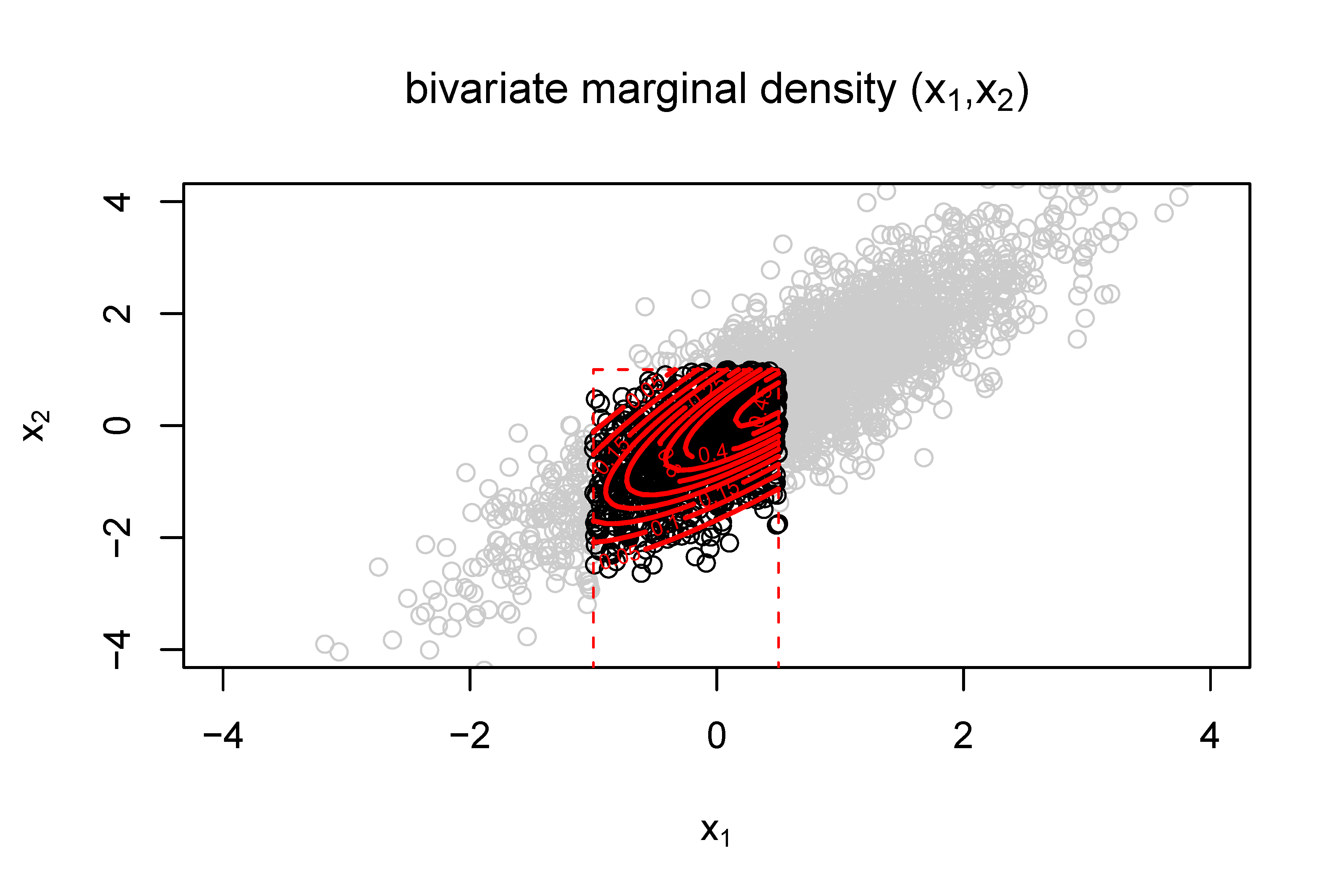
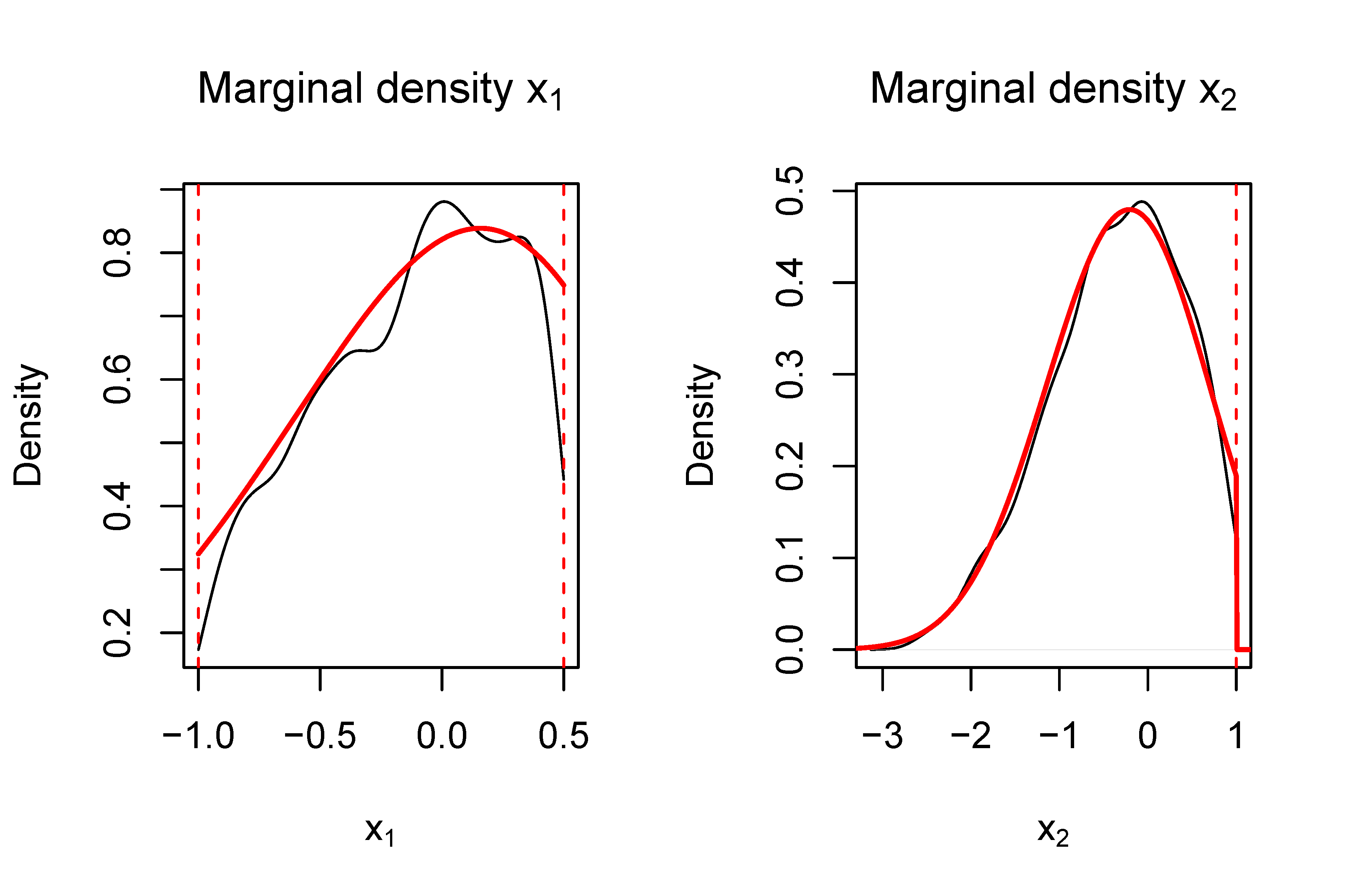
4 Bivariate Marginal Density Computation

In order to compute the bivariate marginal density in this section, we follow Tallis (1961, p. 223) and Leppard and Tallis (1989) that implicitly used the bivariate marginal density as part of the moments calculation for single truncation, evaluated at the integration bounds. However, we extend it to the doubly truncated case and state the function for all points within the support region.

Without loss of generality we use a z-transformation for all variates $\bfx = (x_1,\ldots ,x_d)'$ as well as for all lower and upper truncation points $\bfa = (a_1, \ldots , a_d)'$ and $\bfb = (b_1,\ldots ,b_d)'$, resulting in a $N(0,\bfR )$ distribution with correlation matrix $\bfR $ for the standardized untruncated variates. In this section we treat all variables as if they are z-transformed, leaving the notation unchanged.

For computing the bivariate marginal density $F_{q,r}(x_q,x_r)$ with $a_q\le x_q \le b_q, a_r\le x_r \le b_r, q \ne r$, we use the fact that for truncated normal densities the conditional densities are also truncated normal. The following relationship holds for $x_s,z_s \in \mathbb {R}^{d-2}$ conditionally on $x_q = c_q$ and $x_r = c_r$ $(s \ne q \ne r)$:

where and $\bfR _{qr}$ is the matrix of the second-order partial correlation coefficients for $s \ne q \ne r$. $\beta _{sq.r}$ and $\beta _{sr.q}$ are the partial regression coefficients of $x_s$ on $x_q$ and $x_r$ , respectively, and $\rho _{sr.q}$ is the partial correlation coefficient between $x_s$ and $x_r$ for fixed $x_q$.

Integrating out $(d-2)$ variables $x_s$ leads to $F_{q,r}(x_q,x_r)$ as a product of a bivariate normal density $\varphi (x_q,x_r)$ and a $(d-2)$-dimension normal integral $\Phi _{d-2}$:

where $A^q_{rs}$ and $B^q_{rs}$ denote the lower and upper integration bounds of $\Phi _{d-2}$ given $x_q=c_q$ and $x_r=c_r$: The computation of $F_{q,r}(x_q,x_r)$ just needs the evaluation of the normal integral $\Phi _{d-2}$ in $d-2$ dimensions, which is readily available in most statistics software packages, for example, as the function pmvnorm() in the R package mvtnorm (Genz et al., 2012). The bivariate marginal density function dtmvnorm(x, mean, sigma, lower, upper, margin=c(q,r)) is also part of the R package tmvtnorm (Wilhelm & Manjunath, 2010, 2012), where readers can find the source code as well as help files and additional examples.

5 Numerical Examples

Example 1

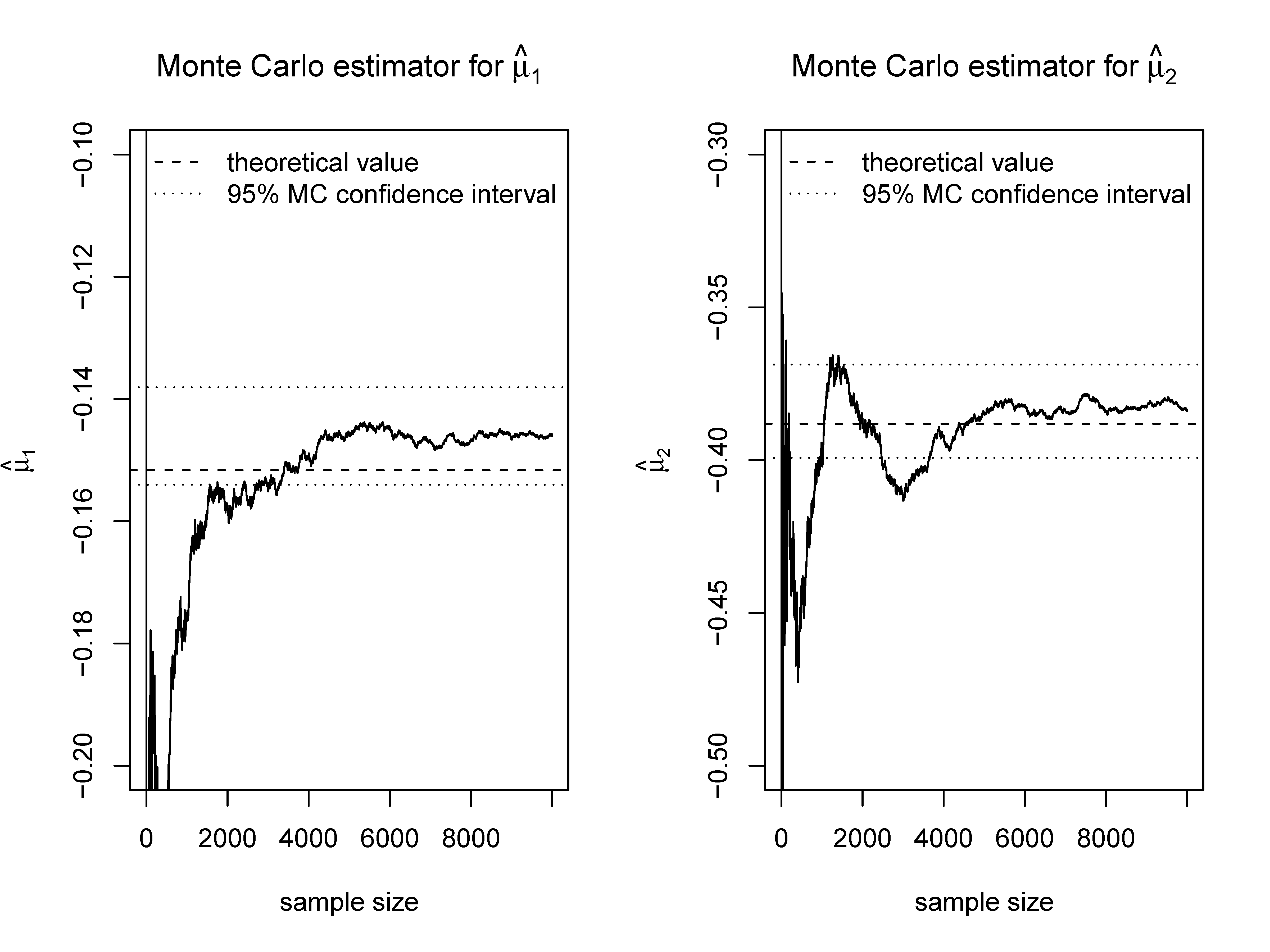
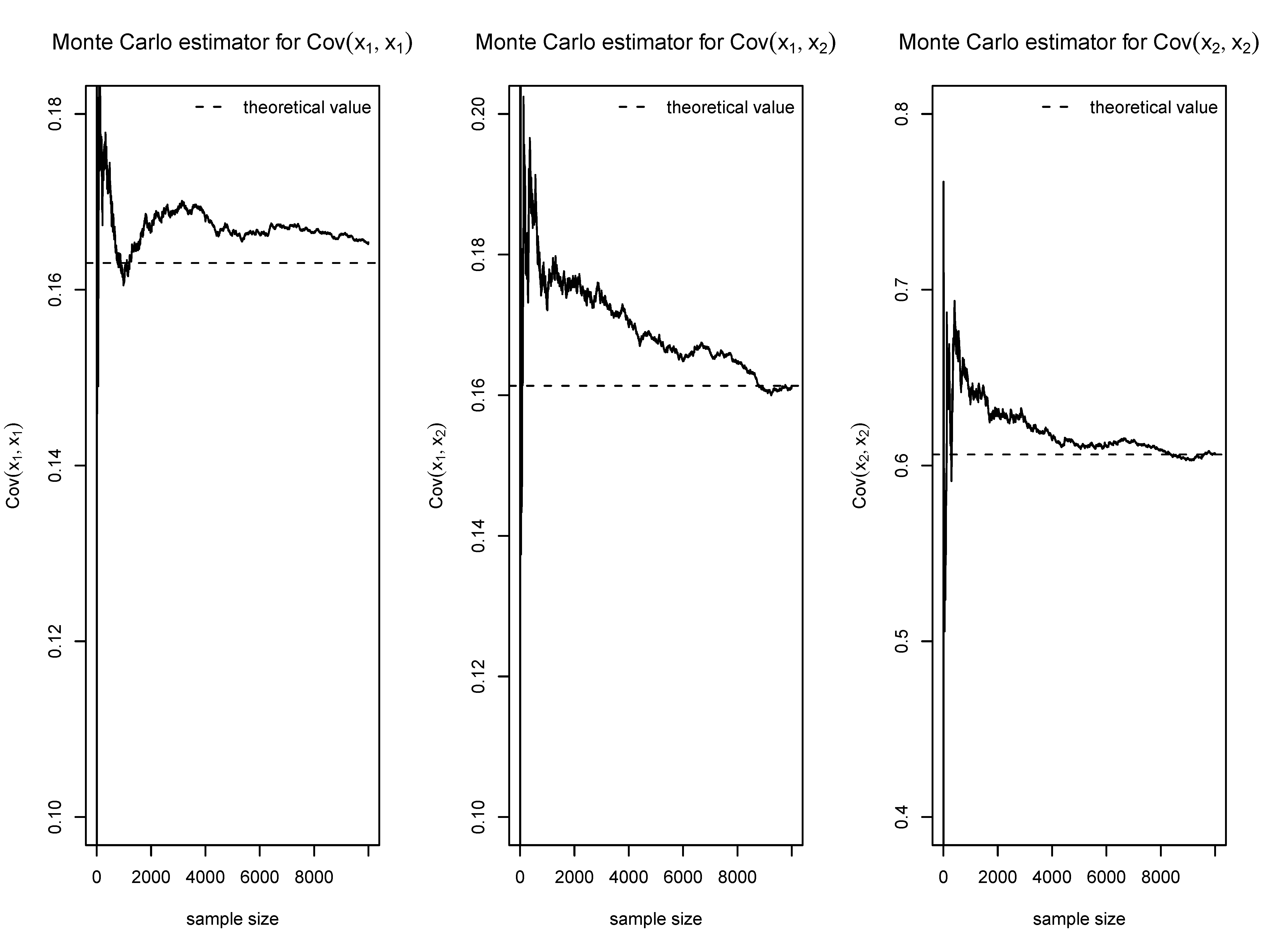
We will use the following bivariate example with $\bfmu = (0.5, 0.5)'$ and covariance matrix $\bfSi $

as well as lower and upper truncation points $\bfa =(-1, -\infty )',\bfb = (0.5, 1)'$, i.e. $x_1$ is doubly, while $x_2$ is singly truncated. The bivariate marginal density $F_{q,r}(x,y)$ is the density function itself and is shown in figure 1, and the one-dimensional densities $F_k(x)$ ($k=1,2$) are shown in in figure 2.

---

---

---

---

The moment calculation for our example can be performed in R as

which leads to the results $\bfmu ^{*} = (-0.152, -0.388)'$ and covariance matrix

The trace plots in figures 3 and 4 show the evolution of a Monte Carlo estimate for the elements of the mean vector and the covariance matrix respectively for growing sample sizes. Furthermore, the 95% confidence interval obtained from Monte Carlo using the full sample of 10000 items is shown. All confidence intervals contain the true theoretical value, but Monte Carlo estimates still show substantial variation even with a sample size of 10000. Simulation from a truncated multivariate distribution and calculating the sample mean or the sample covariance also leads to consistent estimates of $\bfmu ^{*}$ and $\bfSi ^{*}$. Since the rate of convergence of the MC estimator is $O(\sqrt {n})$, one has to ensure sufficient Monte Carlo iterations in order to have a good approximation or to choose variance reduction techniques.

---

---

---

---

Example 2

Let $\bfmu = (0, 0, 0)'$,the covariance matrix

and the lower and upper truncation points $\bfa =(-1, -\infty , -\infty )'$ and $\bfb = (0.5, \infty , \infty )'$. Then the only truncated variable is $x_1$, which is uncorrelated with $x_3$. Our formula results in $\bfmu ^{*} = c(-0.210, -0.229, 0)'$ and For the special case of only $k < d$ truncated variables $(x_1, \ldots , x_k)$, the remaining $d-k$ variables $(x_{k+1}, \ldots , x_d)$ can be regressed on the truncated variables, and a simple formula for the mean and covariance matrix can be given (see Johnson & Kotz, 1971, p. 70).

Let the covariance matrix $\bfSi $ of $(x_1,\ldots , x_d)$ be partitioned as

where $\bfV _{11}$ denotes the $k \times k$ covariance matrix of $(x_1, \ldots , x_k)$. The mean vector¹ and the covariance matrix $\bfSigma ^*$ of all $d$ variables can be computed as and where $\boldsymbol {\xi '_1}$ and $\bfU _{11}$ are the mean and covariance of the $(x_1, \ldots , x_k)$ after truncation.

The mean and standard deviation for the univariate truncated normal $x_1$ are

Letting $\bfU _{11} = \sigma _{11}^{*}$ and inserting $\xi _1$ and $\bfU _{11}$ into equations (25) and (26), one can verify our formula and the results for $\bfmu ^{*}$ and $\bfSi ^{*}$. However, the crux in using the Johnson/Kotz formula is the need to first compute the moments of the truncated variables $(x_1, \ldots , x_k)$ for $k \ge 2$. But this has been exactly the subject of our paper.

6 Moment Calculation and Conditional Independence

In this section we establish a link between our moment calculation and the theory of graphical models (Edwards, 1995; Lauritzen, 1996; Whittaker, 1990). We present some properties of the inverse covariance matrix and show how the dependence structure of variables is affected after selection.

Graphical modeling uses graphical representations of variables as nodes in a graph and dependencies among them as edges. A key concept in graphical modeling is the conditional independence property. Two variables $x$ and $y$ are conditionally independent given a variable or a set of variables $z$ (notation $x \ci y | z$), when $x$ and $y$ are independent after partialling out the effect of $z$. For conditionally independent $x$ and $y$, the edge between them in the graph is omitted and the joint density factorizes as $f(x, y | z) = f(x | z) f(y | z)$.

Conditional independence is equivalent to having zero elements $\bfOmega _{xy}$ in the inverse covariance matrix $\bfOmega = \bfSigma ^{-1}$ as well as having a zero partial covariance/correlation between $x$ and $y$ given the remaining variables: \[ x \ci y | \text {Rest} \iff \bfOmega _{xy} = 0 \iff \rho _{xy.Rest} = 0. \] Both marginal independence and conditional independence between variables simplify the computations of the truncated covariance in equation (16). In the presence of conditional independence of $i$ and $j$ given $q$, the terms $\sigma _{ij} - \sigma _{iq} \sigma ^{-1}_{qq} \sigma _{qj} = 0$ vanish as they reflect the partial covariance of $i$ and $j$ given $q$.

As has been shown by Marchetti and Stanghellini (2008), the conditional independence property is preserved after selection, i.e. the inverse covariance matrices $\bfOmega $ and $\bfOmega ^*$ before and after truncation share the same zero-elements.
We prove that many elements of the precision matrix are invariant to truncation. For the case of $k < d$ truncated variables, we define the set of truncated variables with $T=\{x_1, \ldots , x_k\}$, and the remaining $d-k$ variables as $S=\{x_{k+1}, \ldots , x_d\}$. We can show that the off-diagonal elements $\bfOmega _{i,j}$ are invariant after truncation for $i \in T \cup S$ and $j \in S$:
Proposition 1. The off-diagonal elements $\bfOmega _{i,j}$ and the diagonal elements $\bfOmega _{j,j}$ are invariant after truncation for $i \in T \cup S$ and $j \in S$.

Proof. The proof is a direct application of the Johnson/Kotz formula in equation (26) in the previous section. As a result of the formula for partitioned inverse matrices (Greene, 2003, section A.5.3) , the corresponding inverse covariance matrix $\bfOmega $ of the partitioned covariance matrix $\bfSigma $ is

with $\bfF _2 = (\bfV _{22} - \bfV _{21} \bfV _{11}^{-1} \bfV _{12})^{-1}$.

Inverting the truncated covariance matrix $\bfSigma ^*$ in equation (26) using the formula for the partitioned inverse leads to the truncated precision matrix

where the $\bfOmega ^*_{12}$ and $\bfOmega ^*_{21}$ elements are the same as $\bfOmega _{12}$ and $\bfOmega _{21}$ respectively. The same is true for the elements in $\bfOmega ^*_{22}$, especially the diagonal elements in $\bfOmega ^*_{22}$. $\square $

Here, we prove this invariance property only for a subset of truncated variables. Based on our experiments we conjecture that the same is true also for the case of full truncation (i.e. all off-diagonal elements in $\bfOmega ^*_{11}$). However, we do not give a rigorous proof here and leave it to future research.

Example 3

We illustrate the invariance of the elements of the inverse covariance matrix with the famous mathematics marks example used in Whittaker (1990) and Edwards (1995, p. 49). The independence graph of the five variables $(W, V, X,$ $Y, Z)$ in this example takes the form of a butterfly as shown in below.

---

---

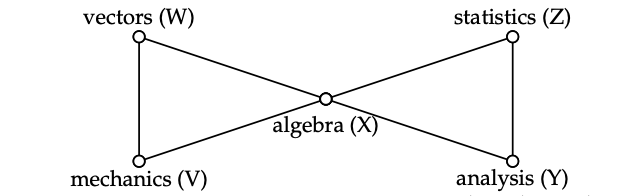
Here, we have the conditional independence $(W, V) \ci (Y, Z) | X$. A corresponding precision matrix might look like (sample data; zero-elements marked as ”.”):

After truncation in some variables (for example $(W, V, X)$ as $-2 \le W \le 1$, $-1 \le V \le 1$, $0 \le X \le 1$), we apply equation (16) to compute the truncated second moment and the inverse covariance matrix as:

The precision matrix $\bfOmega ^*$ after selection differs from $\bfOmega $ only in the diagonal elements of $(W, V, X)$. From $\bfOmega ^*$, we can read how partial correlations between variables have changed due to the selection process.

Each diagonal element $\bfOmega _{yy}$ of the precision matrix is the inverse of the partial variance after regressing on all other variables (Whittaker, 1990, p. 143). Since only those diagonal elements in the precision matrix for the $k \le d$ of the truncated variables will change after selection, this leads to the idea to just compute these $k$ elements after selection rather than the full $k(k+1)/2$ symmetric elements in the truncated covariance matrix and applying the Johnson/Kotz formula for the remaining $d-k$ variables. However, the inverse partial variance of a scalar $y$ given the remaining variables $X=\{x_1,\ldots ,x_d\} \setminus {y}$ \[ \bfOmega^*_{yy} = \left[ \Sigma^{*}_{y.X} \right]^{-1} = \left[ \Sigma^{*}_{yy} - \Sigma^{*}_{yX} \Sigma^{*-1}_{XX} \Sigma^{*}_{Xy} \right]^{-1} \] still requires the truncated covariance results derived in Section 3.

7 Summary

In this paper, we derived a formula for the first and second moments of the doubly truncated multivariate normal distribution and for their bivariate marginal density. An implementation for both formulas has been made available in the R statistics software as part of the tmvtnorm package. We linked our results to the theory of graphical models and proved an invariance property for elements of the precision matrix. Further research can deal with other types of truncation (e.g. elliptical). Another line of research can look at the moments of the doubly truncated multivariate Student-t distribution, which contains the truncated multivariate normal distribution as a special case.

References

Open Access Statement. Journal of Behavioral Data Science, ISSN 2575-8306, online ISSN 2574-1284. © International Society for Data Science and Analytics. All content of the Journal of Behavioral Data Science is freely available to download, save, reproduce, and transmit for noncommercial, scholarly, and educational purposes. Reproduction and transmission of journal content for the above purposes should credit the author and original source. Use, reproduction, or distribution of journal content for commercial purposes requires additional permissions from the International Society for Data Science and Analytics; please contact contact@isdsa.org. DOI: 10.35566/jbds

References

Amemiya, T. (1974). Multivariate regression and simultaneous equations models when the dependent variables are truncated normal. Econometrica, 42, 999–1012. doi: https://doi.org/10.2307/1914214
Arellano-Valle, R. B., & Genton, M. G. (2005). On fundamental skew distributions. Journal of Multivariate Analysis, 96, 93–116. doi: https://doi.org/10.1016/j.jmva.2004.10.002
Arismendi, J. C. (2013). Multivariate truncated moments. Journal of Multivariate Analysis, 117, 41–75. doi: https://doi.org/10.1016/j.jmva.2013.01.007
Cartinhour, J. (1990). One-dimensional marginal density functions of a truncated multivariate normal density function. Communications in Statistics - Theory and Methods, 19, 197–203. doi: https://doi.org/10.1080/03610929008830197
Edwards, D. (1995). Introduction to graphical modelling. Springer.
Galarza C.E., R., Kan, & V.H., L. (2021). MomTrunc: Moments of folded and doubly truncated multivariate distributions. Retrieved from https://cran.r-project.org/web/packages/MomTrunc (R package version v5.97)
Genz, A. (1992). Numerical computation of multivariate normal probabilities. Journal of Computational and Graphical Statistics, 1, 141–149. doi: https://doi.org/10.2307/1390838
Genz, A., Bretz, F., Miwa, T., Mi, X., Leisch, F., Scheipl, F., & Hothorn, T. (2012). mvtnorm: Multivariate normal and t distributions. Retrieved from http://CRAN.R-project.org/package=mvtnorm (R package version 0.9-9992)
Greene, W. H. (2003). Econometric analysis (5th ed.). Prentice-Hall.
Gupta, A. K., & Tracy, D. S. (1976). Recurrence relations for the moments of truncated multinormal distribution. Communications in Statistics - Theory and Methods, 5(9), 855–865. doi: https://doi.org/10.1080/03610927608827402
Johnson, N. L., & Kotz, S. (1971). Distributions in statistics: Continuous multivariate distributions. John Wiley & Sons.
Kan, R., & Robotti, C. (2017). On moments of folded and truncated multivariate normal distributions. Journal of Computational and Graphical Statistics, 26(4), 930–934. doi: https://doi.org/10.1080/10618600.2017.1322092
Lauritzen, S. (1996). Graphical models. Oxford University Press.
Lee, L.-F. (1979). On the first and second moments of the truncated multi-normal distribution and a simple estimator. Economics Letters, 3, 165–169. doi: https://doi.org/10.1016/0165-1765(79)90111-3
Lee, L.-F. (1983). The determination of moments of the doubly truncated multivariate tobit model. Economics Letters, 11, 245–250.
Leppard, P., & Tallis, G. M. (1989). Algorithm AS 249: Evaluation of the mean and covariance of the truncated multinormal distribution. Applied Statistics, 38, 543–553. doi: https://doi.org/10.2307/2347752
Marchetti, G. M., & Stanghellini, E. (2008). A note on distortions induced by truncation with applications to linear regression systems. Statistics & Probability Letters, 78, 824–829. doi: https://doi.org/10.1016/j.spl.2007.09.050
Muthen, B. (1990). Moments of the censored and truncated bivariate normal distribution. British Journal of Mathematical and Statistical Psychology, 43, 131–143. doi: https://doi.org/10.1111/j.2044-8317.1990.tb00930.x
Regier, M. H., & Hamdan, M. A. (1971). Correlation in a bivariate normal distribution with truncation in both variables. Australian Journal of Statistics, 13, 77–82. doi: https://doi.org/10.1111/j.1467-842x.1971.tb01245.x
Rosenbaum, S. (1961). Moments of a truncated bivariate normal distribution. Journal of the Royal Statistical Society. Series B (Methodological), 23, 405-408. doi: https://doi.org/10.1111/j.2517-6161.1961.tb00422.x
Shah, S. M., & Parikh, N. T. (1964). Moments of single and doubly truncated standard bivariate normal distribution. Vidya (Gujarat University), 7, 82–91.
Tallis, G. M. (1961). The moment generating function of the truncated multinormal distribution. Journal of the Royal Statistical Society, Series B (Methodological), 23(1), 223–229. doi: https://doi.org/10.1111/j.2517-6161.1961.tb00408.x
Tallis, G. M. (1963). Elliptical and radial truncation in normal populations. The Annals of Mathematical Statistics, 34(3), 940–944. doi: https://doi.org/10.1214/aoms/1177704016
Tallis, G. M. (1965). Plane truncation in normal populations. Journal of the Royal Statistical Society, Series B (Methodological), 27(2), 301–307. doi: https://doi.org/10.1111/j.2517-6161.1965.tb01497.x
Whittaker, J. (1990). Graphical models in applied multivariate statistics. John Wiley & Sons.
Wilhelm, S., & Manjunath, B. G. (2010, June). tmvtnorm: A Package for the Truncated Multivariate Normal Distribution. The R Journal, 2(1), 25–29. doi: https://doi.org/10.32614/rj-2010-005
Wilhelm, S., & Manjunath, B. G. (2012). tmvtnorm: Truncated multivariate normal distribution and Student t distribution. Retrieved from http://CRAN.R-project.org/package=tmvtnorm (R package version 1.4-5)
1 The formula for the truncated mean given in Johnson and Kotz (1971, p. 70) is only valid for a zero-mean vector or after demeaning all variables appropriately. For non-zero means $\bfmu =(\bfmu _1, \bfmu _2)'$ it will be $(\boldsymbol {\xi '_1}, \bfmu _2 + (\boldsymbol {\xi '_1} - \bfmu _1) \bfV ^{-1}_{11} \bfV _{12})$.